gghighlight 0.2.0 – Wannabe Rstats-fu

gghighlight 0.2.0 is on CRAN a while ago. This post briefly introduces the three new features. For basic usages, please refer to “Introduction to gghighlight”.

`keep_scales`

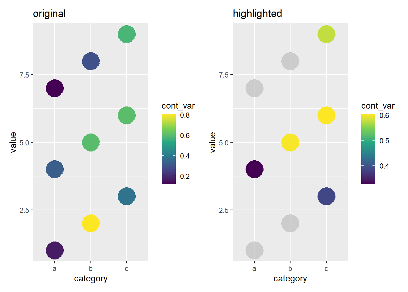
To put it simply, gghighlight doesn’t drop any data points but drops their colours. This means, while non-colour scales (e.g. x, y and size) are kept as they are, colour scales get shrinked. This might be inconvenient when we want to compare the original version and the highlighted version, or the multiple highlighted versions.

library(gghighlight)

Loading required package: ggplot2

library(patchwork)

set.seed(3)

d <- data.frame(
  value = 1:9,
  category = rep(c("a","b","c"), 3),
  cont_var = runif(9),
  stringsAsFactors = FALSE
)

p <- ggplot(d, aes(x = category, y = value, color = cont_var)) +
  geom_point(size = 10) +
  scale_colour_viridis_c()

p1 <- p + ggtitle("original")
p2 <- p + 
  gghighlight(dplyr::between(cont_var, 0.3, 0.7),
              use_direct_label = FALSE) +
  ggtitle("highlighted")

Warning: Tried to calculate with group_by(), but the calculation failed.
Falling back to ungrouped filter operation...

p1 * p2

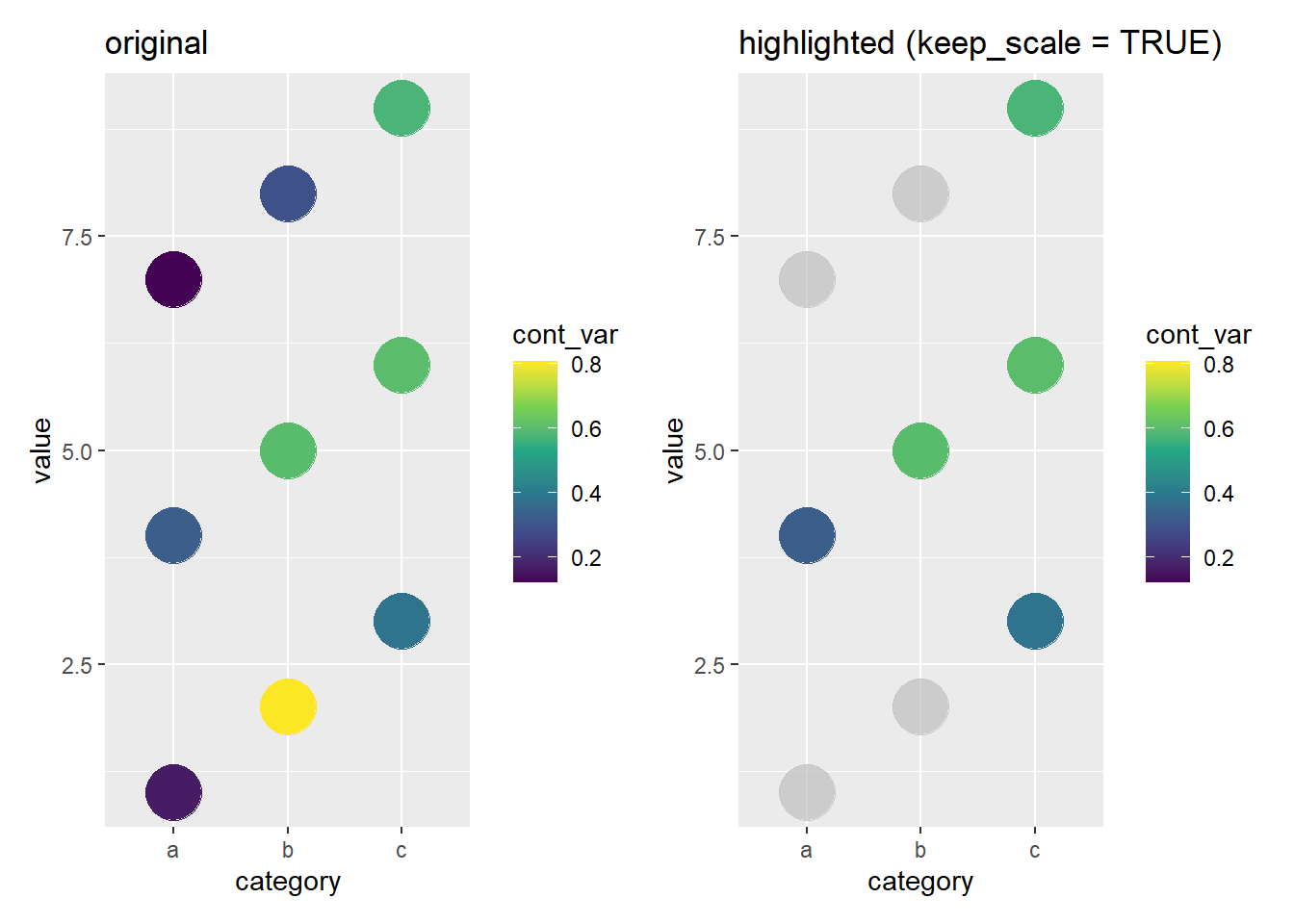
You can see the colour of the points are different between the left plot and the right plot because the scale of the colours are different. In such a case, you can specify keep_scale = TRUE to keep the original scale (under the hood, gghighlight simply copies the original data to geom_blank()).

p3 <- p +
  gghighlight(dplyr::between(cont_var, 0.3, 0.7),
              keep_scales = TRUE,
              use_direct_label = FALSE) +
  ggtitle("highlighted (keep_scale = TRUE)")

Warning: Tried to calculate with group_by(), but the calculation failed.
Falling back to ungrouped filter operation...

p1 * p3

`calculate_per_facet`

When used with facet_*(), gghighlight() puts unhighlighted data on all facets and calculate the predicates on the whole data.

Sys.setlocale(locale = "C")

[1] "C"

set.seed(16)

d <- tibble::tibble(
  day = rep(as.Date("2020-01-01") + 0:89, times = 4),
  month = lubridate::ceiling_date(day, "month"),
  value = c(
    cumsum(runif(90, -1.0, 1.0)),
    cumsum(runif(90, -1.1, 1.1)),
    cumsum(runif(90, -1.1, 1.0)),
    cumsum(runif(90, -1.0, 1.1))
  ),
  id = rep(c("a", "b", "c", "d"), each = 90)
)

p <- ggplot(d) +
  geom_line(aes(day, value, colour = id)) +
  facet_wrap(~ month, scales = "free_x")

p + 
  gghighlight(mean(value) > 0, keep_scales = TRUE)

label_key: id

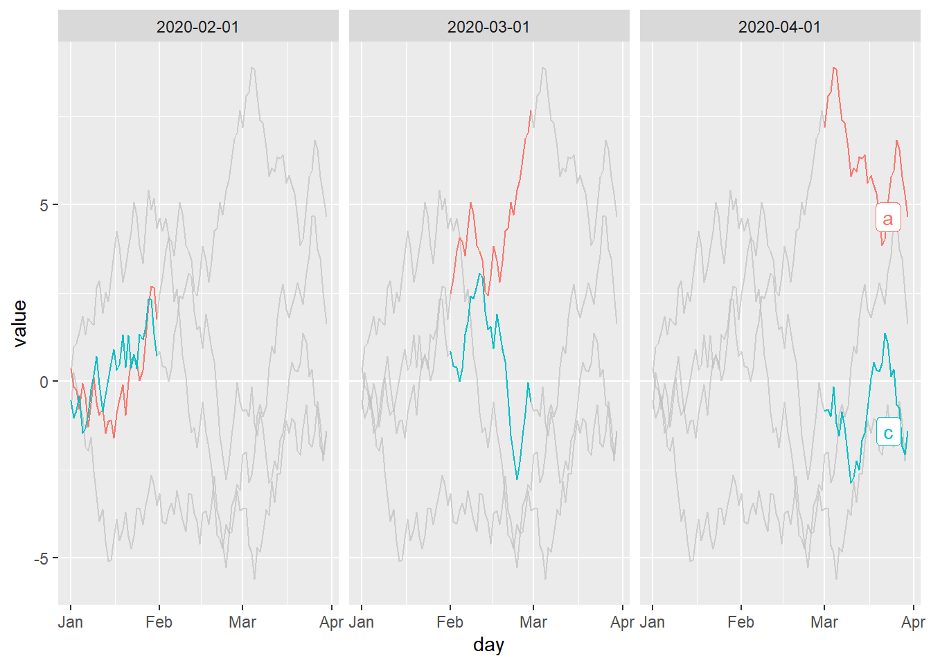
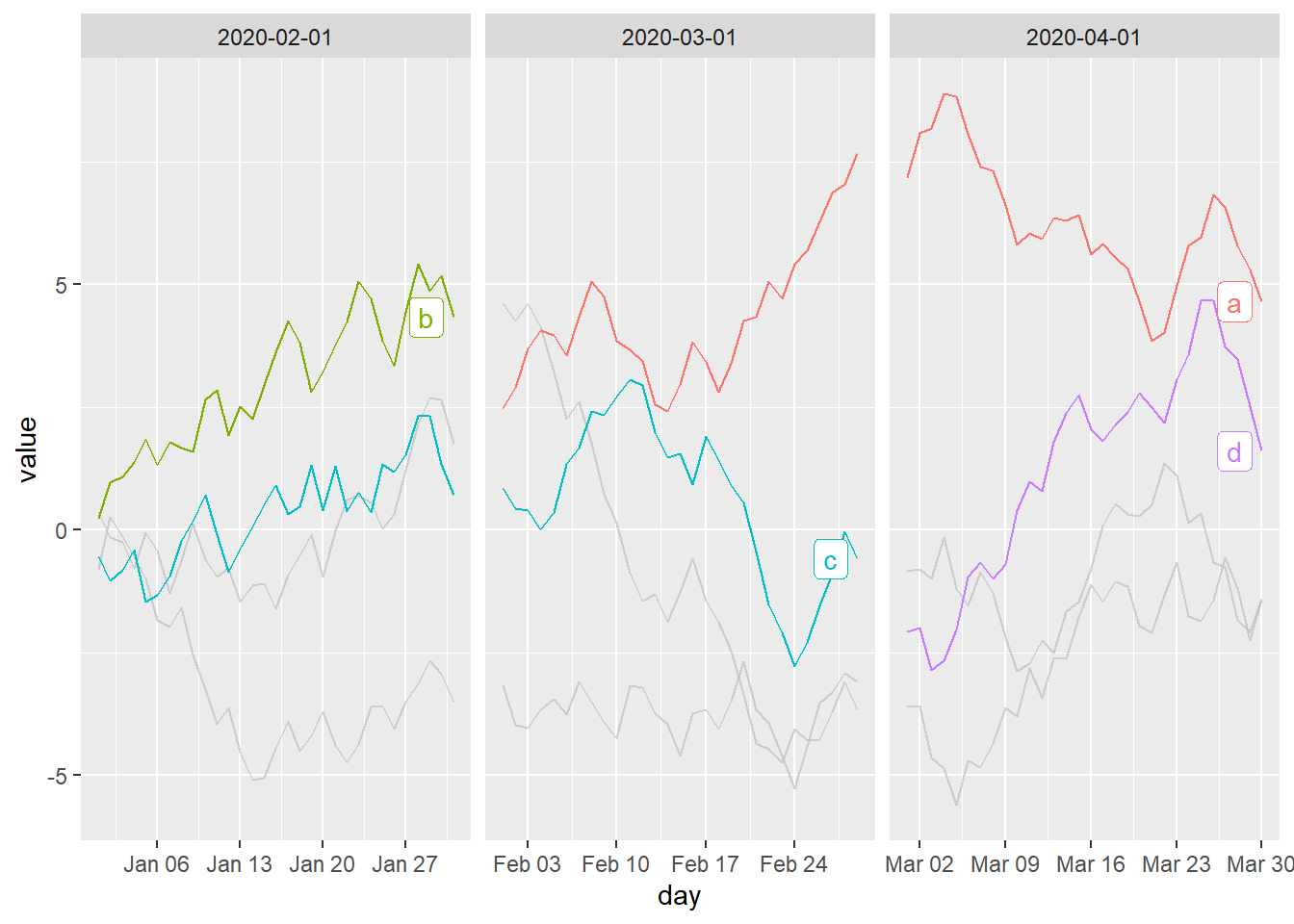
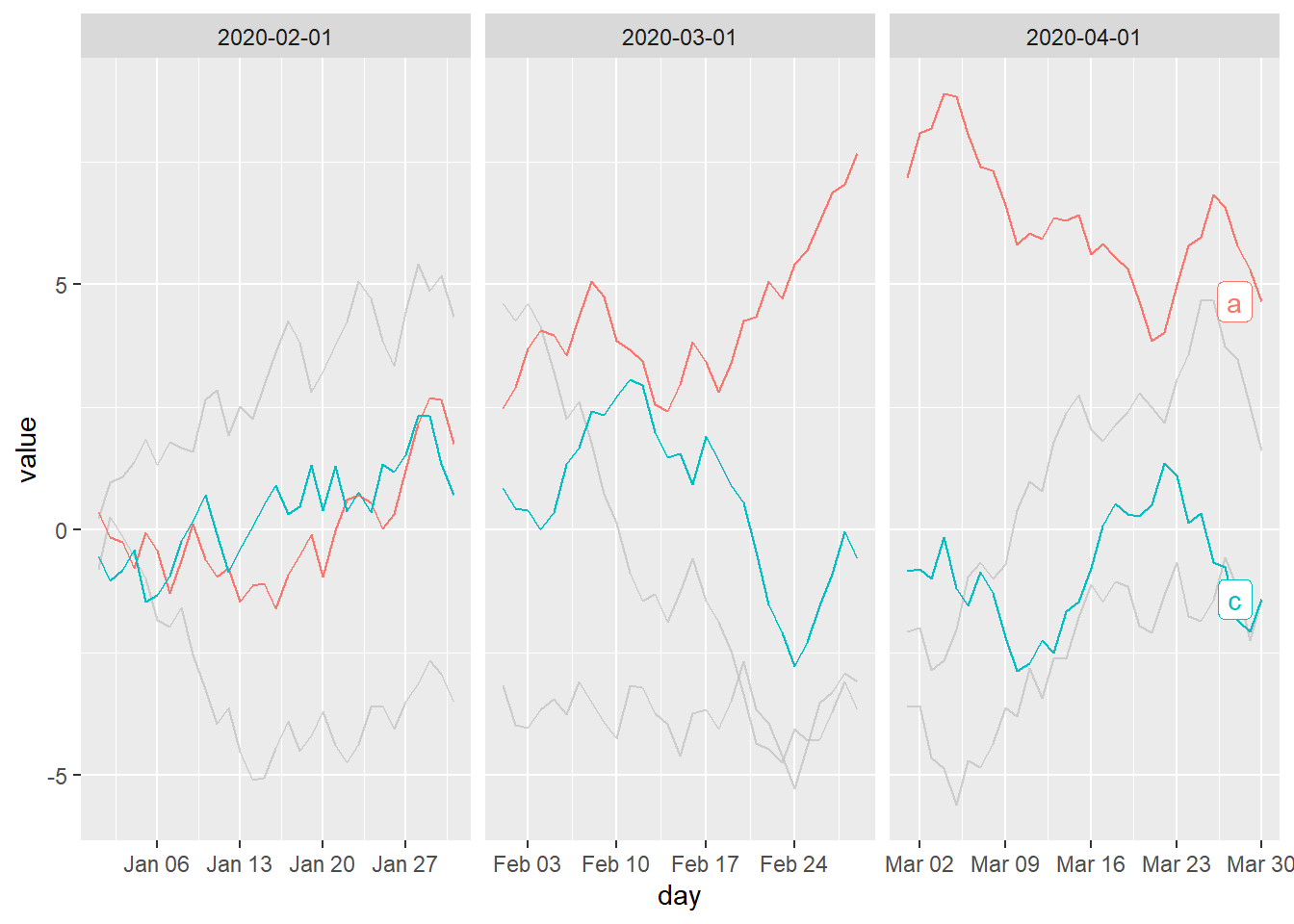
But, it sometimes feels better to highlight facet by facet. For such a need, gghighlight() now has a new argument calculate_per_facet.

p + 
  gghighlight(mean(value) > 0,
              calculate_per_facet = TRUE,
              keep_scales = TRUE)

label_key: id

Note that, as a general rule, only the layers before adding gghighlight() are modified. So, if you add facet_*() after adding gghighlight(), this option doesn’t work (though this behaviour might also be useful in some cases).

ggplot(d) +
  geom_line(aes(day, value, colour = id)) +
  gghighlight(mean(value) > 0,
              calculate_per_facet = TRUE,
              keep_scales = TRUE) +
  facet_wrap(~ month, scales = "free_x")

label_key: id

`unhighlighted_params`

gghighlight() now allows users to override the parameters of unhighlighted data via unhighlighted_params. This idea was suggested by @ClausWilke.

I think you could support a broader set of use cases if you allowed a list of aesthetics default values, like bleach_aes = list(colour = "grey40", fill ="grey80", size = 0.2).

— Claus Wilke (@ClausWilke) July 4, 2018

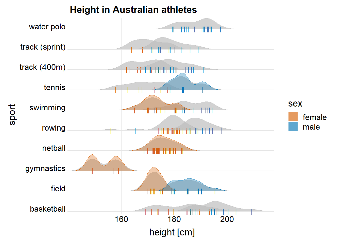
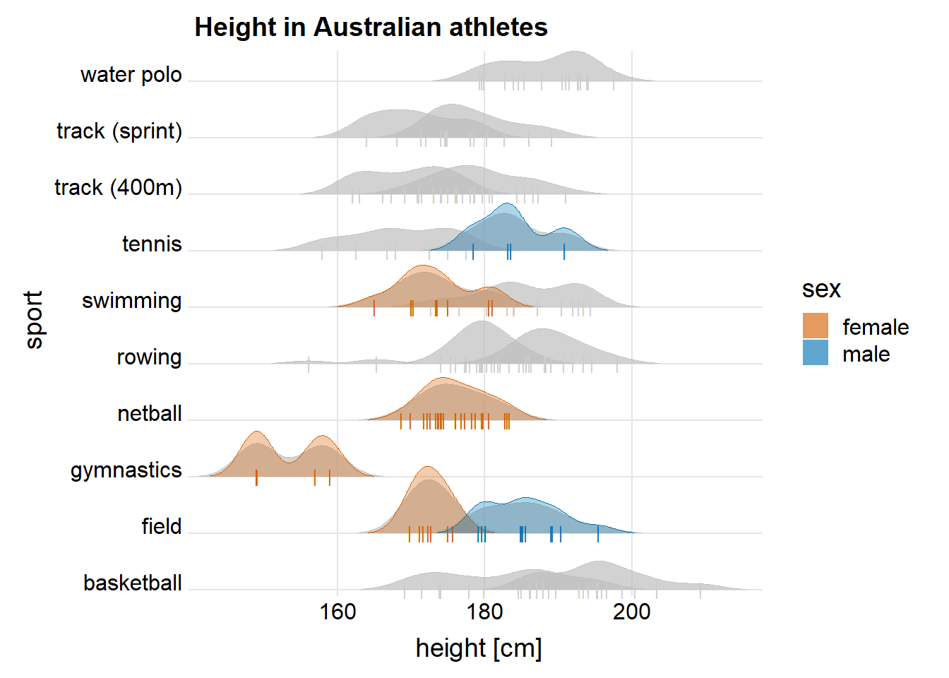
To illustrate the original motivation, let’s use an example on the ggridges’ vignette. gghighlight can highlight almost any Geoms, but it doesn’t mean it can “unhighlight” arbitrary colour aesthetics automatically. In some cases, you need to unhighlight them manually. For example, geom_density_ridges() has point_colour.

library(ggplot2)
library(gghighlight)
library(ggridges)

p <- ggplot(Aus_athletes, aes(x = height, y = sport, color = sex, point_color = sex, fill = sex)) +
  geom_density_ridges(
    jittered_points = TRUE, scale = .95, rel_min_height = .01,
    point_shape = "|", point_size = 3, size = 0.25,
    position = position_points_jitter(height = 0)
  ) +
  scale_y_discrete(expand = c(0, 0)) +
  scale_x_continuous(expand = c(0, 0), name = "height [cm]") +
  scale_fill_manual(values = c("#D55E0050", "#0072B250"), labels = c("female", "male")) +
  scale_color_manual(values = c("#D55E00", "#0072B2"), guide = "none") +
  scale_discrete_manual("point_color", values = c("#D55E00", "#0072B2"), guide = "none") +
  coord_cartesian(clip = "off") +
  guides(fill = guide_legend(
    override.aes = list(
      fill = c("#D55E00A0", "#0072B2A0"),
      color = NA, point_color = NA)
    )
  ) +
  ggtitle("Height in Australian athletes") +
  theme_ridges(center = TRUE)

p + 
  gghighlight(sd(height) < 5.5)

Picking joint bandwidth of 2.8

Picking joint bandwidth of 2.23

You should notice that these vertical lines still have their colours. To grey them out, we can specify point_colour = "grey80" on unhighlighted_params (Be careful, point_color doesn’t work…).

p + 
  gghighlight(sd(height) < 5.5, 
              unhighlighted_params = list(point_colour = "grey80"))

Picking joint bandwidth of 2.8

Picking joint bandwidth of 2.23

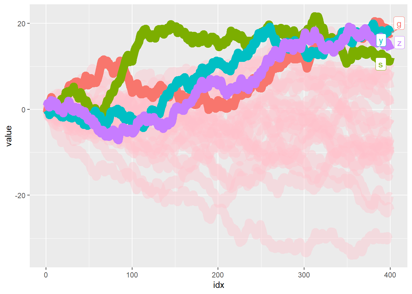
unhighlighted_params is also useful when you want more significant difference between the highlighted data and unhighligted ones. In the following example, size and colour are set differently.

set.seed(2)
d <- purrr::map_dfr(
  letters,
  ~ data.frame(
      idx = 1:400,
      value = cumsum(runif(400, -1, 1)),
      type = .,
      flag = sample(c(TRUE, FALSE), size = 400, replace = TRUE),
      stringsAsFactors = FALSE
    )
)

ggplot(d) +
  geom_line(aes(idx, value, colour = type), size = 5) +
  gghighlight(max(value) > 19,
              unhighlighted_params = list(size = 1, colour = alpha("pink", 0.4)))

size aesthetic has been deprecated for use with lines as of ggplot2 3.4.0
i Please use linewidth aesthetic instead
label_key: type

This message is displayed once every 8 hours.